Formatting

Excel has a number of formatting options on the Home tab, including:

1. Font effects like font families, colours, underlines, ect
2. Cell effects like size, borders, merging, and colours
3. Text effects like wrapping and alignment
4. Formatting options, like Currency, Percentages, and Numbers
5. Conditional Formatting

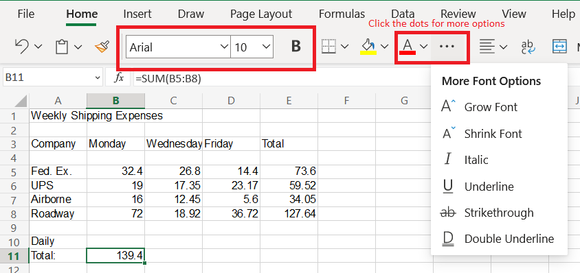
Font Effects

To change your font options, select the cell or cells you want to change, then select from the options you what you want to add.

1. To change the font family or size, select them from the drop downs. What you place in the dropdown will be automatically applied
2. To make the cell bold, italicized, or underlined, click on the associated icon. For underlines on the web version, you will need to click the dots for "more font options"
3. To change the font colour, select the colour from the drop down, select the cells you want to apply it to, then click on the capital A above it to apply it

Cell Effects

Applying cell effects is similar to font effects.

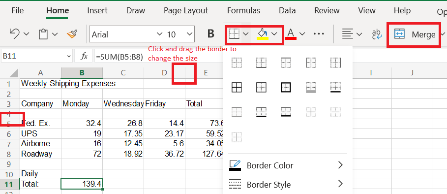
1. You can change cell sizes by clicking on the edges of the column number or row letter and dragging it the direction you want to change
2. To apply borders, select from the border options which you would like to apply (usually all borders) and what colour you would like the border to be, select the cells you would like to apply them to, and click the borders icon to apply it
3. To merge cells, which removes the borders allowing one cell to span across many rows or columns, write the value you want to merge into the top left cell. Then, select the range of cells you would like to merge and click the "Merge" button. Only the value in the top left cell will be kept
4. To change the cell background colour, pick the colour you would like, select the cells you would like to change, then click the fill paint bucket

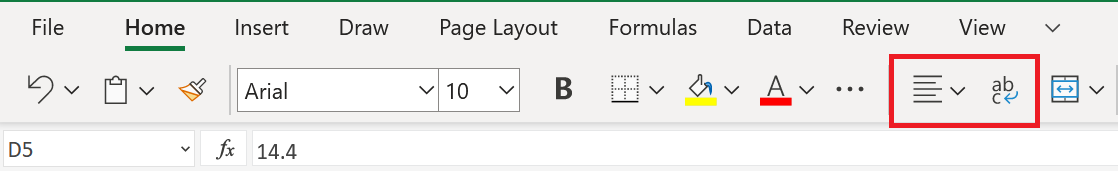
Text Effects

1. Text wrapping will send text down into the next line instead of bleeding into the cell to the right. To enable this, select the cell you want to wrap and click "Wrap"
2. Text alignment changes what part of the cell the text will be written to. Usually be default text is placed on the left and numbers on the right, but if you would like to change this, just select the cells you want to change and then click which justification you would like

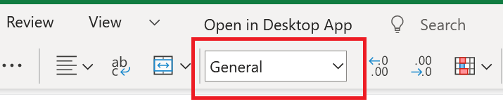
Formatting Options

To change how data is displayed, select the cells and choose from the drop down, such as currency. Please note that changing the format may change the way some functions interact with the data in the cells.

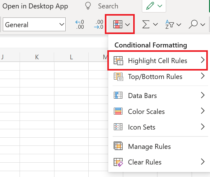
Conditional Formatting

Perhaps the most useful formatting option is conditional formatting. Conditional formatting will change the appearance of a cell depending on what values are in it, such as green for above 0 and red for below 0. There are a lot of more complicated things you can do, but we won't cover them in this class.

1. Select the cells you want to conditionally format
2. Select the "Conditional" drop down, then "Highlight Cell Rules"


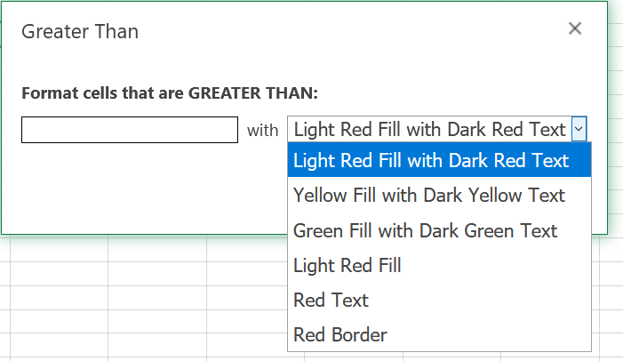
3. Select which criteria you would like to use, such as "Greater Than"
4. Enter the value, then select how you would like cells that meet that criteria to display from the dropdown and click "OK"


5. If you want to set multiple conditions, select the cells again and repeat the process, but choose a different criteria, such as"Less Than," and a different colour