Spreadsheet Exercise #2

• Click here for the spreadsheet needed for this exercise

The following are step by step instructions to complete this spreadsheet.

Step #1: Formatting Text:

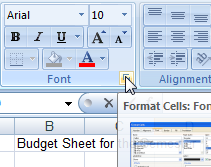
To format the title in the spreadsheet, click on cell B1. Click on the little box in the bottom right of the Font category. Now you should be able to see the menu shown below.

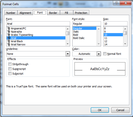
Select Bold, change the color to blue and change the font size to 16. Click on OK when you are done.

Excel gives you a toolbar along the top of the screen to simplify many formatting commands. Let's make use of this toolbar to do more formatting. To format the column headers, select cells A3 to F3 by holding the left mouse button and dragging it across from A3 to F3. Click on the B (Bold) button in the center of the toolbar. Then click on the drop down list box the left of the toolbar so you can change the font size. Select 12 from the dropdown list.

Let's kick this up another notch by doing an even simpler format of all of the column A cells. Click on the A button at the top of the worksheet to select the entire column. Now use the toolbar to make all of that column Bold and 12 point size.

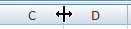
Now there's a problem that's not obvious here. Column A is not wide enough for all of the labels in its cells. You need to position your cursor over the boundary between column A and column B and wait till you see the little "adjust" icon appear. Drag the cursor to the right until all of the labels in the Column A cells are visible.

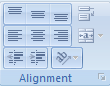
Now, just one more formatting task for the labels, highlight the cells B3 to F3 and then click on the "Right Align" button from the set of alignment buttons on the toolbar.

Step #2: Entering Data:

Most of the data has already been entered. There are just a few more entries to make, and then we can use some of Excel's functions to complete the rest of the spreadsheet.

• To enter the monthly income for September, select cell B15, type the number 2700, and press the Enter key. Don't worry about getting in the dollar signs, commas, and periods just yet.
• To enter the monthly income for October, select the next cell, C15, type the number 700 and press the Enter key.
• Now the rest of the monthy incomes can all be set to the same as October, so the easy way to do that is:
• Click on the October income.
• Drag right to highlight the November and December incomes.
• Go to the Editing menu, and select Fill Right.
• Before you proceed, highlight all of the cells that will contain dollar values (B5 to F17) and click on the dollar sign icon found in the currency area.

Step #3: Entering Formulas:

Don't forget to use the = sign before entering a formula.
The letters do not need to be capital letters.

• The first formula will go into cell F5. Select that cell and enter the following formula: =SUM(B5:E5)
  Press the Enter key to signal that you have completed the formula.
• Now copy that formula down the column to F11. Do this by highlighting F5 to F11, and then click on the Editing menu and select Fill Down.
• The second formula will go into cell B13. Select that cell and enter the following formula: =SUM(B5:B11)
• Now copy that formula across the row to E13. Do this by highlighting B13 to E13., and then click on the Editing menu and select Fill Right.
• To enter the formula for the September Monthly Balance, select cell B17 and enter the following formula: =B15-B13
• The next formula builds on that somewhat because you want to include the balance from the previous month in your calculation. Select cell C17 and enter this formula: =(C15-C13)+B17
• Now copy that formula across the row to E17. Do this by highlighting C17 to E17, and then click on the Editing menu and select Fill Right.


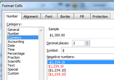
• You should really set up the format for the monthly balances(cells B17:E17) differently than the other cells. Highlight these cells, go to the Format menuand click on the Number tab, select the Currency option and select the fourth option under "Negative Numbers".
  To test this out, go to cell D11 and enter $600.

Step #4: Entering an IF Function:

• Let's place a row below the Monthly Balance row that indicates if your current balance is "OK", or if you are "Overdrawn". The cells in that row can be implemented by an IF function.
• First you will need to select cell B18 by clicking on it.
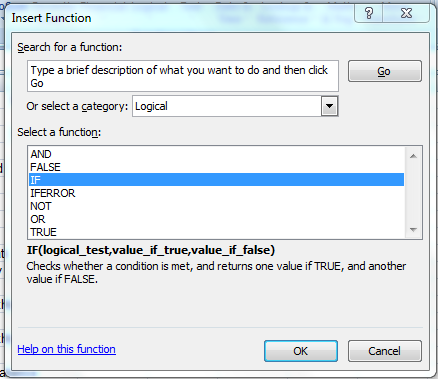
• Select the Formulas tab and then click on Insert Function. Click on the category for Logical functions. Now you should see the dialogue box shown above.
• Look at the requirements of the IF function. These are called the arguments to the function. You need to specify the condition, B17>=0, then the value "OK", then the value "Overdrawn". Separate these things by commas, and because the OK and Overdrawn are text, you need to type in the quotation marks i.e. "OK", "Overdrawn" Don't forget the equal sign for the formula, and the parentheses around the arguments to the function. When you are finished, this is how the formula with the IF function should appear:
  =IF(B17>=0,"OK","Overdrawn")
  Notice the quotation marks around the words OK and Overdrawn.If you had wanted numbers there instead of words, you would drop the quotation marks.
• To duplicate that IF statement over the row, highlight cells B18 to E18 and then select Editing and Fill Right
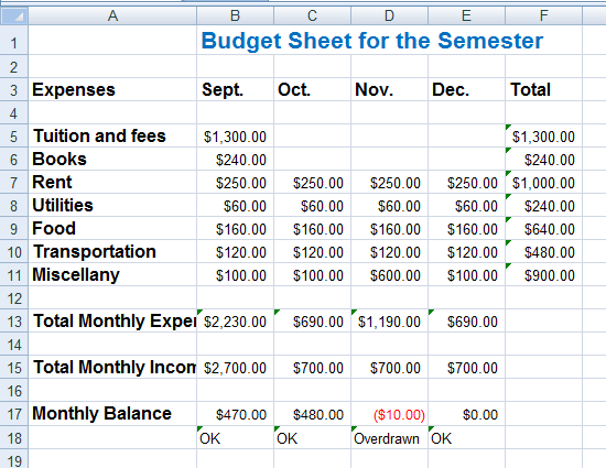
• Notice rows 17 and 18 in particular. You should see a negative value in red and encased in parentheses in cell D17. Just below that you should see the word "Overdrawn". All of the other balances are fine, so the word "OK" appears beneath them. This results from the IF function.

Now you should be finished editing your spreadsheet and it should look something like this: