Spreadsheet Exercise #3

For this exercise, we will use the spreadsheet loans2:

• Click on loans2.xlsx for an Excel version of the spreadsheet
• Save the file to your Documents folder

The following are step by step instructions to complete this spreadsheet.

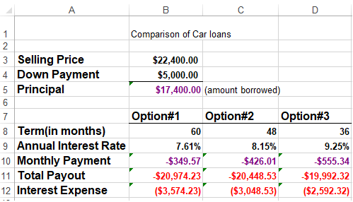
This exercise gives you practice in using spreadsheets, but it also demonstrates how a spreadsheet can be used to assist people in decision making. e.g. You are about to purchase a car and are confused by all the payment options. You can enter formulas into a spreadsheet so that you can see the total cost for each option. The goal of this exercise is to produce a spreadsheet that looks something like this:

Step #1: Formatting Text:

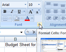
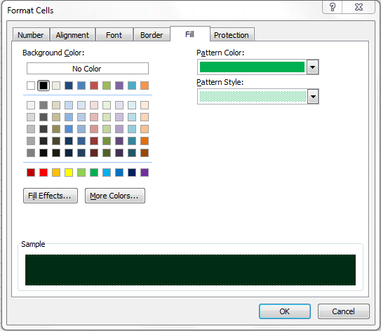
Select cell B1, C1 and D1 by holding the left mouse button and dragging it across from B1 to D1. Open the Format menu previously discussed. Select Underline and Bold, change the color and change the font size to 16.

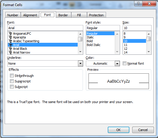
You will notice the word Fill on one of the tabs; click on it. Now select a Pattern Style from the menu list and select a Pattern Colour. Click on OK when you are done.

Step #2: Entering Data:

• Select cell B3 and type the number 22400 and press the Enter key.
  This is the selling price.
• Select cell B4 and type the number 5000 and press the Enter key.
  This is the down-payment amount.
  

Step #3: Entering Formulas: (Absolute and Relative References)

• The first formula will go into cell B5. Select that cell and enter the following formula: =B3-B4
• The second formula will go into cell B12. Select that cell and enter the following formula: =B11+$B$5
• Select the cells B12, C12 and D12 by selecting cell B12 and dragging the cursor to D12.
• Now click on the Editing menu and select Fill Right.
1. You will notice the dollar sign ($) in the second formula. This is an absolute reference. No matter where you copy the formula to it will always refer back to that specific cell (B5 in this case).
2. In the first formula, there were no dollar signs ($). This is refered to as a relative reference. If this formula is copied to a different cell, the formula will change its cell references accordingly.

Don't forget to use the = sign before entering a formula.
The letters do not need to be capital letters.

Step #4: Entering a Function:

The first function that we will use is a financial function. It will determine the monthly payment for us.

• First you will need to select cell B10 by clicking on it.
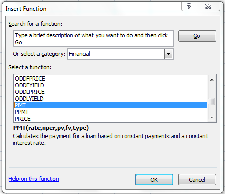
• Select the Formulas tab and then click on Insert Function. Now you should see the following menu.


• Select the financial category and select the PMT function.
• Press OK
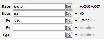
• Fill the fields in so it looks like the following picture.


• Select cells B10, C10 and D10 and then select Editing and Fill Right

The next formula that we will use is a multiplication formula. It will multiply two cells for us.

• Select cell B11
• Type in the following: =B10*B8
  The asterisk (*) is the multiplication symbol.
• Select the cells B11, C11 and D11 and then select Editing and Fill Right

Step #5: Changing Data to Currency:

There are two possible ways to do this:

#1

• Click and hold the left mouse button on cell B10 and drag it to cell D11.
  Now you should have a range of cells selected from B10 to D11 (B10:D11).
• Now click on the currency icon along the top toolbar.

OR

#2

• Click and hold the left mouse button on cell B10 and drag it to cell D11.
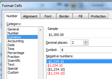
  Now you should have a range of cells selected from B10 to D11 (B10:D11).
• Click on Format and select Number and that should bring up the following menu.
  Select the currency format type along the left side and then enter the number of decimal places you desire.
  (usually two is sufficient).
• Press OK

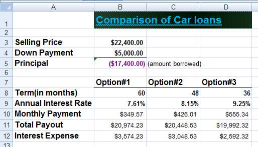
Now you should be finished editing your spreadsheet and it should look something like this: