CS315: Illumination 2

Highlights of this lab:

1. The Blinn-Phong equation revisited
2. Distance and Positional Lights
3. Hemisphere lighting

Assignment:

• Add Blinn-Phong Specular Lighting code from the lab example shader to the exercise code.
• Add distance based attenuation to your positional lights.
• Complete the code I started for you so you have multiple lights at once.
• Move lighting calculations and modify varyings between the vertex and fragment shaders to achieve Phong shading and get smooth highlights.
• Create and name a material of your own.

Lab Notes

Start with the files from Lab5.zip.

In last week's lab you saw these pictures. They show a full implementation of the Blinn-Phong reflection equation being applied in three different ways. The first is flat shading - one colour is used for one whole primitive (triangle). The second is Gouraud shading - reflection is only calculated at the vertices, and colours are interpolated. The last is Phong shading - the full lighting equation is performed per fragment in the fragment shader. This week you will see results that look like all three columns, but you will always be doing Gouraud shading. You will add the Blinn-Phong specular component to a vertex shader, which produces the whitish highlight you see. The smoothness or flatness you will observe will be created entirely in the model - either by using the same normal for all vertices of a primitive (flat-like results) or high resolution meshes (Phong-like results).

Flat Shading	Gouraud Shading	Phong Shading

Figure 1:Torus at different resolutions lit with Blinn-Phong reflection and shaded with different shading models.

A. Blinn-Phong Equation Revisited

When you start to work with lighting, you move beyond color to normals, material properties and light properties. Normals describe what direction a surface is facing at a particular point. Material properties describe of what things are made of — or at least what they appear to be made of — by describing how they reflect light. Light properties describe the type and colour of the light interacting with the materials in the scene. Lights and materials can interact in many different ways. Describing these many different ways is one reason shaders are so important to modern 3D graphics APIs.

One common lighting model that relates geometry, materials and lights is the Blinn-Phong reflection model. It breaks lighting up into three simplified reflection components: diffuse, specular and ambient reflection. In this week's lab we will focus on specular reflection. The other two are left here for your reference.

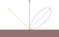
Specular Reflection

Specular reflection represents the shine that you see on very smooth or polished surfaces. Phong specular reflection takes into account both the angle between your eye and the direction the light would be reflected. As your eye approaches the direction of reflection, the apparent brightness increases. It assumes that light will be scattered toward the mirror reflection direction. A special shininess parameter is used to control how tight this scattering is. The Blinn-Phong specular reflection is very similar to Phong, but it fixes some technical shortcomings having to do with backscatter (compare the curves you see if figure 5). Instead of using the reflection vector it uses a vector that is halfway between the light and the eye. This vector is then compared to the normal.

The Blinn-Phong specular component is calculated by these equations:

h = (e+l)/|(e+l)|
I_s = m_s L_s (h · n)^s

Where:

• I_s is the intensity of specular reflection
• m_s is the material's specular colour
• L_s is the light's specular colour
• l is the normalized direction to the light
• e is the normalized direction to the eye
• n is the surface normal
• s is the exponent that controls shininess.

	Specular exponent
	1	10	100
Phong
Blinn-Phong

Figure 2: Phong vs Blinn-Phong With Varying Shininess Values.
Both the Phong and Blinn-Phong reflectance functions cause a highlight to appear around the direction of reflection. Blinn-Phong has a fix that allows a near-diffuse disctribution at low shininess. Notice that at shininess 1 the Phong highlight would be invisible past 90° from the reflection direction, but Blinn-Phong is visible well past that point. Blinn-Phong also appears slightly more diffuse at all shininess values than Phong.

Putting Things Together

This specular colour is added to the diffuse and ambient colours described in last week's lab. The illumination of an object from one light, then, is the sum of each of these components.

I = I_s + I_d + I_a

//diffuse and ambient multi-light shader

//inputs
attribute vec4 vPosition;
attribute vec3 vNormal;

//outputs
varying vec4 color;

//structs
struct _light
{
    vec4 diffuse;
    vec4 ambient;
    vec4 specular;
    vec4 position;
};

struct _material
{
    vec4 diffuse;
    vec4 ambient;
    vec4 specular;
    float shininess;
};

//constants
const int nLights = 1; // number of lights

//uniforms
uniform mat4 p;     // perspective matrix
uniform mat4 mv;    // modelview matrix
uniform bool lighting;  // to enable and disable lighting
uniform vec4 uColor;    // colour to use when lighting is disabled
uniform _light light[nLights]; // properties for the n lights
uniform _material material;    // material properties

//globals
vec4 mvPosition; // unprojected vertex position
vec3 N; // fixed surface normal

//prototypes
vec4 lightCalc(in _light light);

void main() 
{
  //Transform the point
  mvPosition = mv*vPosition;  //mvPosition is used often
  gl_Position = p*mvPosition; 

  if (lighting == false) 
  {
	color = uColor;
  }
  else
  {
    //Make sure the normal is actually unit length, 
    //and isolate the important coordinates
    N = normalize((mv*vec4(vNormal,0.0)).xyz);
    
    //Combine colors from all lights
    color.rgb = vec3(0,0,0);
    for (int i = 0; i < nLights; i++)
    {
        color += lightCalc(light[i]);
    }
    color.a = 1.0; //Override alpha from light calculations
  }
}

vec4 lightCalc(in _light light)
{
  //Set up light direction for positional lights
  vec3 L;
  
  //If the light position is a vector, use that as the direction
  if (light.position.w == 0.0) 
    L = normalize(light.position.xyz);
  //Otherwise, the direction is a vector from the current vertex to the light
  else
    L = normalize(light.position.xyz - mvPosition.xyz);

  //Set up eye vector
  vec3 E = -normalize(mvPosition.xyz);

  //Set up Blinn half vector
  vec3 H = normalize(L+E); 

  //Calculate specular coefficient
  float Ks = pow(max(dot(N, H),0.0), material.shininess);
  
  //Calculate diffuse coefficient
  float Kd = max(dot(L,N), 0.0);

  //Calculate colour for this light
  vec4 color =  Ks * material.specular * light.specular
               + Kd * material.diffuse * light.diffuse
               + material.ambient * light.ambient;
               
  return color;
}

Appropriate changes should be made to get and set the specular colour and shininess uniforms. The process is similar to what you observed with diffuse and ambient lighting.

Specifying Material Properties

Classic OpenGL has five material properties affect a material's illumination. They are introduced in the Blinn-Phong model section and implemented in the shaders in lab demo 2. They are explained below.

Diffuse and ambient properties:

The diffuse and ambient reflective material properties are a type of reflective effect that is independent of the viewpoint. Diffuse lighting describes how an object reflects a light that is shining on the object. That is, it is how the surface diffuses a direct light source. Ambient lighting describes how a surface reflects the ambient light available. The ambient light is the indirect lighting that is in a scene: the amount of light that is coming from all directions so that all surfaces are equally illuminated by it. Both properties are usually set to the similar colours, though the ambient colour is usually scaled down or darker than the diffuse colour.

Specular and shininess properties:

The specular and the shininess properties of the surface describe reflective effects that are affected by the position of the viewpoint. Specular light is reflected light from a surface that produces the reflective highlights in a surface. The shininess is a value that describes how focused the reflective properties are.

Emissive property:

Emissive light is the light that an object gives off by itself. Objects that represent a light source are typically the only objects that you give an emissive value. Lamps, fires, and lightning are all objects that give off their own light.

Our shader does not support emissive values as such, but we can simulate it by disabling lighting and using a uniform colour. The light spheres in this week's sample are represented this way.

Choosing the Material Properties for an Object

The steps are as follows:

1. Decide on the diffuse and ambient colors;
2. Decide on the shininess of the object.
3. Decide whether the object is giving off light. If it is, assign it the emissive properties

Seeing the effects of varying material properties may help you select the ones you want.

In this week's first demo - seen below - specular, diffuse and ambient material properties have been implemented. The program provides convenient colour pickers to allow you to select different specular and diffuse/ambient colours interactively. It also provides sliders to rotate the light about the Y-axis and change the shininess value. You should take some time to get familiar with the effects of the different properties. You will be expected to design your own specular material in the exercise after you add specular features to the exercise code.

Click here to view demo on its own.

B. Distance and Positional Lights

In the real world a point light source, or positional light, will have less power to light an object the farther the two are apart. This is called attenuation. Because the light spreads out in an ever increasing sphere, the intensity of the light decreases in inverse proportion to the square of the distance. Classic OpenGL has three parameters to calculate the attenuation factor: constant, linear, and quadratic attenuation. These three factors are used as shown in this equation:

float attenuation = 1.0;
if (/* light is positional */)
{
   float dist = length(light.position.xyz - mvPosition.xyz);
   attenuation = 1.0/(constant + linear * dist + quadratic * dist*dist);
}

This calculation is applied separately to the entire colour of each light - you multiply that light's colour by the attenuation, something like this

// where color is the color result for one light
// and attenuation is 1 for directional lights
color = attenuation * color;

• Constant attenuation is easiest to work with for beginners, and it gives an easy way for you to dim the lights - just crank up the constant attenuation.
• Linear attenuation sometimes gives more natural results if you are not doing HDR tone mapping or some other colour correction.
• Quadratic attenuation is the physically correct term to use, but it causes extreme light differences at short distances, so it is sometimes avoided.

This Desmos graphs can help you visualize the impact of the different coefficients on attenuation with distance and might help you pick coefficients to suit your needs: https://www.desmos.com/calculator/yxblulfnor

Attenuation is not implemented in the shaders in this week's lab. This is left for you to do as an exercise.

C. Hemisphere Lighting

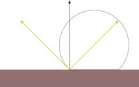
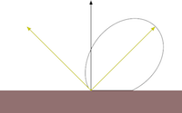
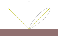
Specular lighting adds a lot to the diffuse and ambient lighting you learned last week. But there's more to add to diffuse lighting. The ambient components are a hack to simulate global illumination, and they do a pretty poor job. Unless you use textures, there's no detail to be seen in ambient light - only a flat silhouette. Hemisphere is a better looking hack that extends the light all around the object. Like diffuse/ambient it uses two light colours, but each is considered to be in opposite hemispheres shining down on the object. Toward the middle, their colours blend smoothly. These colours are intended to represent the sky and the ground, but many implementations allow you to specify the direction of the north pole, or top hemisphere, so it becomes simple to specify, directional, two colour global illumination.

This picture illustrates the intent:

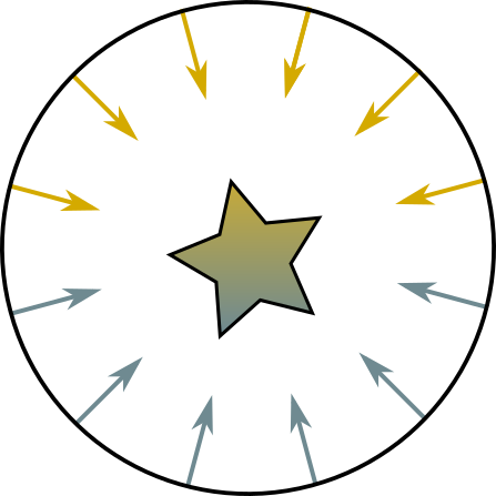Figure 5: Hemisphere lighting's concept. Light falls on the object from two opposite hemispheres and blends across the object.

Downward facing normals are lit entierly by the bottom hemisphere. Upward facing normals are lit entirely by the upper hemisphere. Angled normals are linearly blended (or lerped) between the two based on their angle to the "north pole" or top direction.

The proper equation for this is:

Color = a · TopColor + (1 - a) · BottomColor

Where:

a = 1.0 - (0.5 · sin(Θ)) for Θ ≤ 90°
a = (0.5 · sin(Θ)) for Θ > 90°

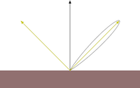
This can be simplified without too much error to:

a = 0.5 + (0.5 · cos(Θ))

Which replaces an expensive sin() with a cos() and saves a branch instruction. Remember, both paths through a branch are always executed in WebGL shader programs. Since this method of global illumination is already approximate, the error is mostly harmless. Here are the two curves overlaid on each other:

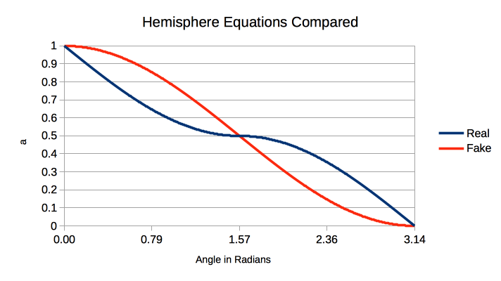Figure 6: Comparison of real vs. fake a calculation for hemisphere lighting.

The following shader implements hemisphere lighting:

//hemisphere lighting shader with optional diffuse lighting path

//inputs
attribute vec4 vPosition;
attribute vec3 vNormal;

//outputs
varying vec4 color;

//structs
struct global_ambient
{
    vec4 direction;  // direction of top colour
    vec4 top;        // top colour
    vec4 bottom;     // bottom colour
};

struct _material
{
    vec4 diffuse;   
};

//uniforms
uniform mat4 p;     // perspective matrix
uniform mat4 mv;    // modelview matrix


uniform _material material; // material properties
uniform global_ambient global;	// global ambient uniform

//globals
vec4 mvPosition; // unprojected vertex position
vec3 N; // fixed surface normal

void main() 
{
  //Transform the point
  mvPosition = mv*vPosition;  //mvPosition is used often
  gl_Position = p*mvPosition; 

  //Make sure the normal is actually unit length, 
  //and isolate the important coordinates
  N = normalize((mv*vec4(vNormal,0.0)).xyz);
    
  //Make sure global ambient direction is unit length
  vec3 L = normalize(global.direction.xyz);
  
  //Calculate cosine of angle between global ambient direction and normal
  float cosTheta = dot(L,N);

  //Calculate global ambient colour
  float a = 0.5+(0.5*cosTheta);
  color = a * global.top * material.diffuse
  	      + (1.0-a)* global.bottom * material.diffuse;
  color.a = 1.0; //Override alpha from light calculations 
                 // (only needs to be done once)
}

And here is a working hemisphere and Lambertian sample for you to experiment with:

Observe how much detail you can make out in the shadows with Hemisphere Lighting as compared with Lambertian Directional Lighting. Notice, also, that the Lambertian blows out the whites if you just increase the brightness of shadows - this is because the ambient and diffuse colours are added rather than linearly blended as with Hemispherical lighting.

Assignment

Start with the files from Lab5.zip. This lab adds two useful libraries - Apple's j3di.js, which provides an OBJ file loader, and East Desire's jscolor.js which provides the colour picker you see in the demos. They are in the lab folder for your convenience. You might want to consider putting copies in the Common folder for your own future use.

If you don't use Visual Studio Code's Live Server extension, Batman - a local .obj file - might not show up in any of the samples. You might need to to start Chrome from a Mac Terminal like this if you want to open local files (like Batman or your own OBJ):

open /Applications/Google\ Chrome.app --args --allow-file-access-from-files

The white ball in the center of the screen is interactive. You can move it side to side and forward and back with the WASD keys. It can also be moved up and down with the Q and E keys. You will enhance this light with specular calculations and distance fading (attenuation). You will also add a second light to the lamp post and make the shiny spots from the lights look nicer with Phong shading. Good luck!!

Goals:

• implement specular lighting calculations in glsl
• understand common attenuation calculations
• learn how to use multiple lights in glsl
• learn how Phong shading is accomplished in glsl
• play with light and material properties to produce a pleasing result

Instructions